1 Day 1 (March 2)
1.1 Welcome
- About the instructors
- Dr. Josefina Lacasa
- Dr. Trevor Hefley
- A bit about our journey to Bayesian models and statistics
1.2 What will we learn?
- Day 1: Introduction to Bayesian modeling
- Two applied examples based on real data
- Coin/phone flip
- Nitrogen balance
- Introduction to statistical modeling
- Introduction to Bayesian models
- Introduction to Bayesian model fitting algorithms (e.g., MCMC) and software (e.g., Stan, JAGS)
- Some finer points about model specification (e.g., priors, likelihood, random effects, etc)
- Two applied examples based on real data
- Day 2: Bayesian modeling of designed experiments
- Review of classical ANOVA
- Introduction to a multilevel approach to ANOVA
- Applied example
- Day 3: Advanced Bayesian modeling of designed experiments
- Review and extension of Bayesian rule to statistical models
- Adaptive design
- Applied example modeling animal weight
- Wrap-up
1.3 Data example 1
Should we flip a coin or a phone?
- Build (specify) the model before we collect data
- Model building philosophy (i.e., the model airplane analogy)
- Download R script here
Likelihood-only inference about p
# The data are...
n <- 5  # Number of flips
y <- 2  # Number of screen landed down

# Maximum likelihood estimate of p with upper and lower 95% Wald-type CI
p.mle <- y/n
p.mle
## [1] 0.4## [1] 0.8294145## [1] -0.02941449Likelihood-only inference about p using glm(…) function
# Doing the same thing as on lines 6-10 but with the glm function
m1 <- glm(cbind(y, n - y) ~ 1, family = binomial(link = "logit"))
summary(m1)
## ## Call: ## glm(formula = cbind(y, n - y) ~ 1, family = binomial(link = "logit")) ## ## Coefficients: ## Estimate Std. Error z value Pr(>|z|) ## (Intercept) -0.4055 0.9129 -0.444 0.657 ## ## (Dispersion parameter for binomial family taken to be 1) ## ## Null deviance: 0 on 0 degrees of freedom ## Residual deviance: 0 on 0 degrees of freedom ## AIC: 4.1249 ## ## Number of Fisher Scoring iterations: 3## 1 ## 0.4## 1 ## 0.8294145## 1 ## -0.02941448Bayesian inference about p
- Bayes rule (Bayes 1763) \[[p|y]=\frac{[y|p][p]}{[y]}\]
- Old school pencil and paper with new school computations (direct sampling…a Monte Carlo method)
# Use direct sampling to obtain 10^6 samples (random draws) from the posterior
# distribution p|y
p.giveny <- rbeta(10^6, y + 1, n - y + 1)
hist(p.giveny, freq = FALSE, main = "Posterior posterior distribution p|y", xlab = "p|y",
    ylab = "[p|y]")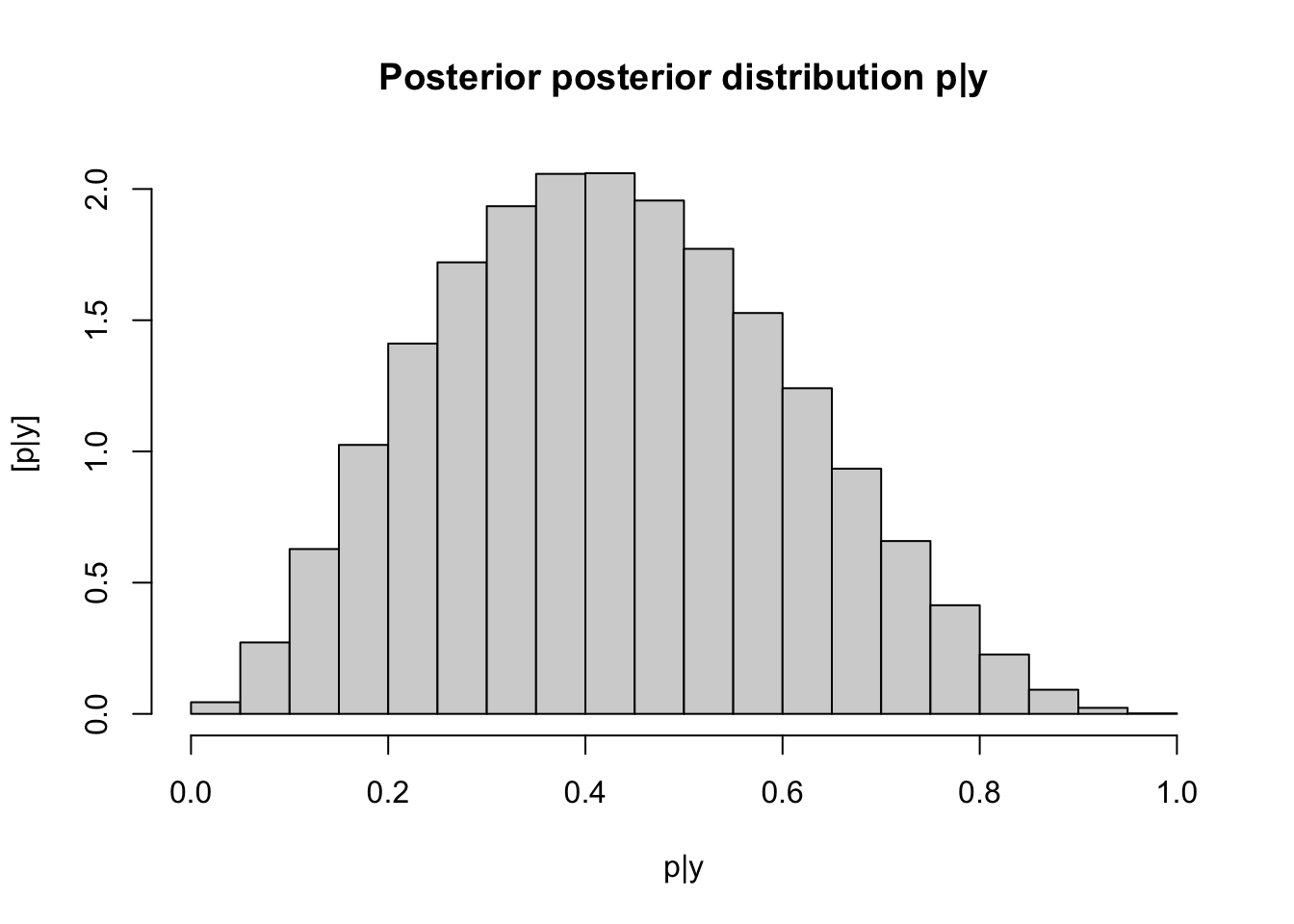
## [1] 0.4287893## 2.5% 97.5% ## 0.1183006 0.7776078Big ideas from this example
- Likelihood-only models works great for medium to high information content data, but may require “small sample size” corrections for low information content data.
- Point estimates are straightforward to obtain, but uncertainty quantification is a bit more tricky
- Bayesian models require more assumptions (e.g., a prior or paramter model), but yield probabilistic inference (i.e., a posterior distribution) and is invariant of sample size
- Regardless of what you do, building a statistical model before you collect the data is critical!
- Likelihood-only models works great for medium to high information content data, but may require “small sample size” corrections for low information content data.
1.4 Data example 2
- What is a linear model?
Most widely used model in science, engineering, and statistics.
Scalar form: \(y_i=\beta_{0}+\beta_{1}x_{i}+\varepsilon_i\)
Which part of the model is the mathematical model.
Which part of the model makes the linear model a “statistical” model.
Visual
1.5 Estimation and inference
- Three options to estimate \(\beta_0\) and \(\beta_1\)
- Minimize a loss function
- Maximize a likelihood function
- Find the posterior distribution
- Each option requires different assumptions
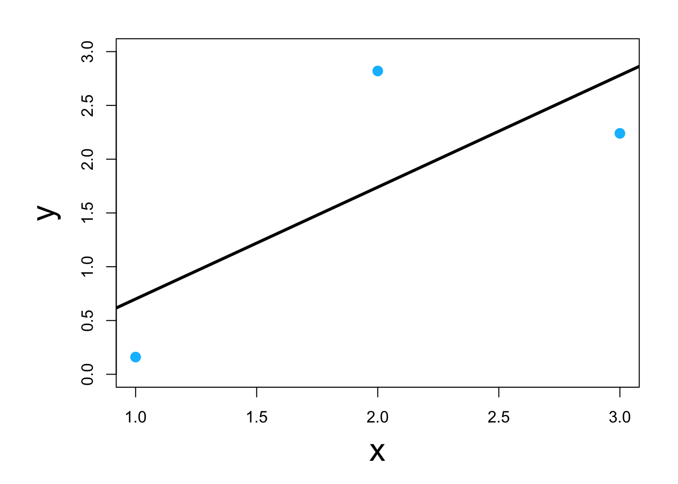
1.6 Loss function approach
- Define a measure of discrepancy between the data and the mathematical model
- Find the values of \(\beta_0\) and \(\beta_1\) that makes \(\beta_{0}+\beta_{1}x_i\) “closest” to \(y_i\)
- Visual
- Real data example
- Details from Palmero et al. (2024)
- Download R script here
# Preliminary steps
url <- "https://www.dropbox.com/scl/fi/2qph4g9vnacibr73edrsb/Fig3_data.csv?rlkey=n48lbrv2zf2z5k1uja1393sof&dl=1"
df.all <- read.csv(url)
df.fp <- df.all[which(df.all$Scenario=="Scenario A"),]

# Plot data for field pea
plot(df.fp$Ndfa,df.fp$PartNbalance,
 xlab="Ndfa (%)",ylab="Partial N balance (kg/ha)",
 xlim=c(0,110),ylim=c(-100,200),main="Field pea")
abline(a=0,b=0,col="gold",lwd=3)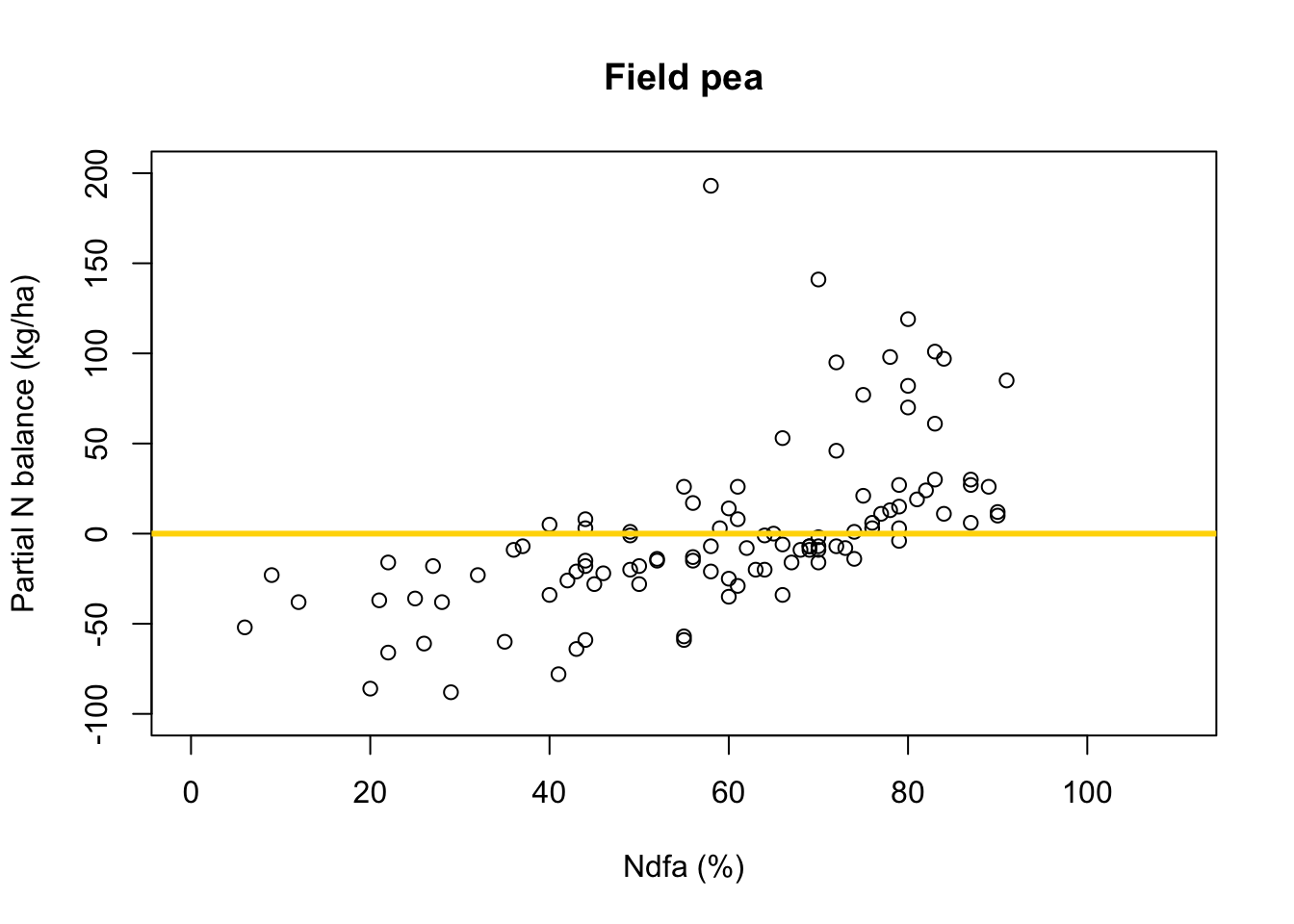
- Fit linear model to data using least squares
- What value of Ndfa is needed to achieve a neutral N balance?
beta0.hat <- as.numeric(coef(m1)[1])
beta1.hat <- as.numeric(coef(m1)[2])
theta.hat <- -beta0.hat/beta1.hat
theta.hat
## [1] 58.26843- Visual representation of \(\theta\)
# Plot data, line of best fit and theta
plot(df.fp$Ndfa,df.fp$PartNbalance,
 xlab="Ndfa (%)",ylab="Partial N balance (kg/ha)",
 xlim=c(0,110),ylim=c(-100,200),main="Field pea")
abline(a=0,b=0,col="gold",lwd=3)
abline(m1,col="red",lwd=3)
abline(v=58,lwd=3,lty=2,col="green")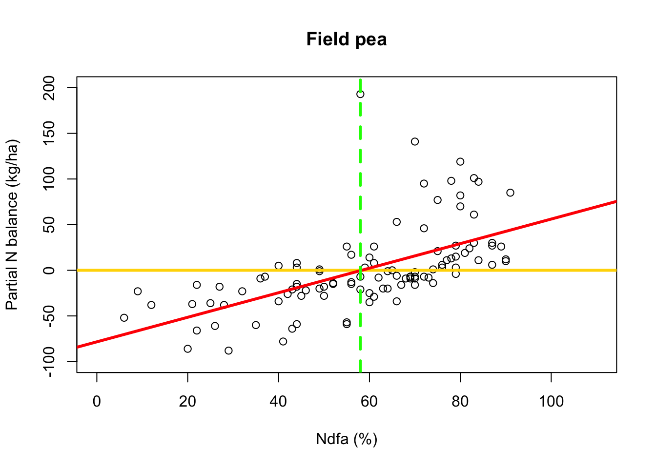
1.7 Likelihood-based approach
- Assume that \(y_i=\beta_{0}+\beta_{1}x_{i}+\varepsilon_i\) and \(\varepsilon_i\sim \text{N}(0,\sigma^2)\)
- Maximum likelihood estimation for the linear model
- Visual
- We added assumptions to our model, so what else do we get?
- Full likelihood-based statistical inference (e.g, p-values, confidence intervals, prediction intervals, etc)
- Real data example
- Fit linear model to data using using maximum likelihood estimation
library(nlme) # Fit simple linear regression model using maximum likelihood estimation m2 <- gls(PartNbalance ~ Ndfa,data=df.fp,method="ML")- What value of Ndfa is needed to achieve a neutral N balance?
# Use maximum likelihood estimate (MLE) to obtain estimate of theta
beta0.hat <- as.numeric(coef(m2)[1])
beta1.hat <- as.numeric(coef(m2)[2])
theta.hat <- -beta0.hat/beta1.hat
theta.hat
## [1] 58.26843# Use delta method to obtain approximate approximate standard errors and # then construct Wald-type confidence intervals library(msm) theta.se <- deltamethod(~-x1/x2, mean=coef(m2), cov=vcov(m2)) theta.ci <- c(theta.hat-1.96*theta.se,theta.hat+1.96*theta.se) theta.ci## [1] 52.88317 63.65370- Visual representation of \(\theta\)
# Plot data, line of best fit and theta
plot(df.fp$Ndfa,df.fp$PartNbalance,
 xlab="Ndfa (%)",ylab="Partial N balance (kg/ha)",
 xlim=c(0,110),ylim=c(-100,200),main="Field pea")
abline(a=0,b=0,col="gold",lwd=3)
abline(m1,col="red",lwd=3)
abline(v=58.3,lwd=3,lty=2,col="green")
abline(v=52.9,lwd=1,lty=2,col="green")
abline(v=63.7,lwd=1,lty=2,col="green")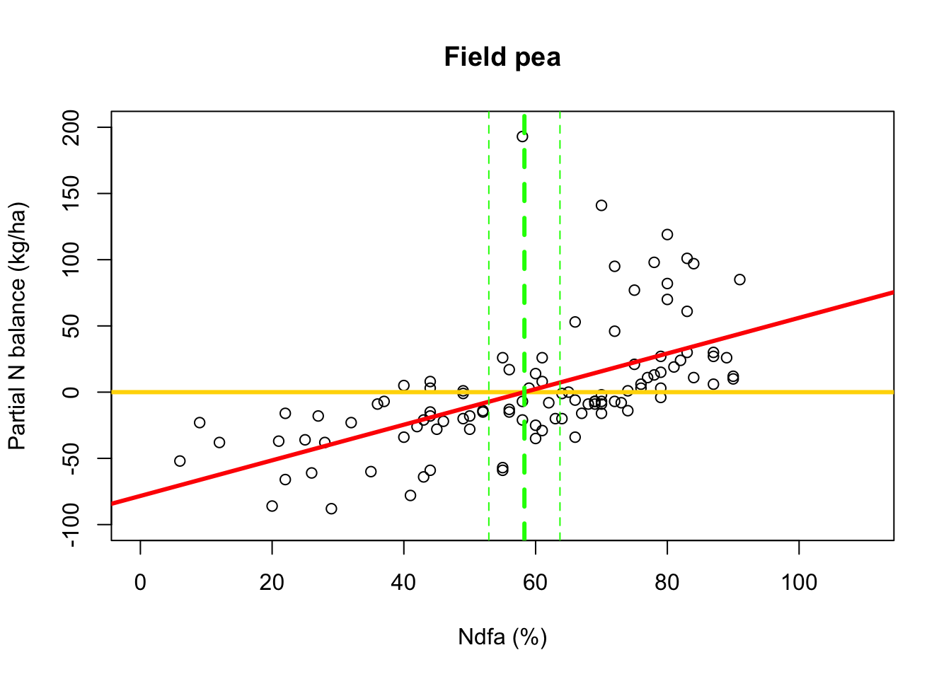
1.8 Bayesian approach
Assume that \(y_i=\beta_{0}+\beta_{1}x_{i}+\varepsilon_i\) with \(\varepsilon_i\sim \text{N}(0,\sigma^2)\), \(\beta_{0}\sim \text{N}(0,10^6)\) and \(\beta_{1}\sim \text{N}(0,10^6)\)
Statistical inference
- Using Bayes rule (Bayes 1763) we can obtain the joint posterior distribution
\[[\beta_0,\beta_1,\sigma_{\varepsilon}^{2}|\mathbf{y}]=\frac{[\mathbf{y}|\beta_0,\beta_1,\sigma_{\varepsilon}^{2}][\beta_0][\beta_1][\sigma_{\varepsilon}^{2}]}{\int\int\int [\mathbf{y}|\beta_0,\beta_1,\sigma_{\varepsilon}^{2}][\beta_0][\beta_1][\sigma_{\varepsilon}^{2}]d\beta_0d\beta_1,d\sigma_{\varepsilon}^{2}}\]
- Statistical inference about a paramters is obtained from the marginal posterior distributions \[[\beta_0|\mathbf{y}]=\int[\beta_0,\beta_1,\sigma_{\varepsilon}^{2}|\mathbf{y}]d\beta_1d\sigma_{\varepsilon}^{2}\] \[[\beta_1|\mathbf{y}]=\int[\beta_0,\beta_1,\sigma_{\varepsilon}^{2}|\mathbf{y}]d\beta_0d\sigma_{\varepsilon}^{2}\] \[[\sigma_{\varepsilon}^{2}|\mathbf{y}]=\int[\beta_0,\beta_1,\sigma_{\varepsilon}^{2}|\mathbf{y}]d\beta_0d\beta_1\]
- Derived quantities can be obtained by transformations of the joint posterior
- Using Bayes rule (Bayes 1763) we can obtain the joint posterior distribution
\[[\beta_0,\beta_1,\sigma_{\varepsilon}^{2}|\mathbf{y}]=\frac{[\mathbf{y}|\beta_0,\beta_1,\sigma_{\varepsilon}^{2}][\beta_0][\beta_1][\sigma_{\varepsilon}^{2}]}{\int\int\int [\mathbf{y}|\beta_0,\beta_1,\sigma_{\varepsilon}^{2}][\beta_0][\beta_1][\sigma_{\varepsilon}^{2}]d\beta_0d\beta_1,d\sigma_{\varepsilon}^{2}}\]
Computations
- Using a Markov chain Monte Carlo algorithm (MCMC; see Ch.11 in Hooten and Hefley 2019)
norm.reg.mcmc <- function(y,X,beta.mn,beta.var,s2.mn,s2.sd,n.mcmc){

  #
  #  Code Box 11.1
  #

  ###
  ### Subroutines
  ###

  library(mvtnorm)

  invgammastrt <- function(igmn,igvar){
q <- 2+(igmn^2)/igvar
r <- 1/(igmn*(q-1))
list(r=r,q=q)
  }

  invgammamnvr <- function(r,q){  #  This fcn is not necessary
mn <- 1/(r*(q-1))
vr <- 1/((r^2)*((q-1)^2)*(q-2))
list(mn=mn,vr=vr)
  }

  ###
  ### Hyperpriors
  ###

  n=dim(X)[1]
  p=dim(X)[2]
  r=invgammastrt(s2.mn,s2.sd^2)$r
  q=invgammastrt(s2.mn,s2.sd^2)$q
  Sig.beta.inv=diag(p)/beta.var

  beta.save=matrix(0,p,n.mcmc)
  s2.save=rep(0,n.mcmc)
  Dbar.save=rep(0,n.mcmc)
  y.pred.mn=rep(0,n)

  ###
  ### Starting Values
  ###

  beta=solve(t(X)%*%X)%*%t(X)%*%y

  ###
  ### MCMC Loop
  ###

  for(k in 1:n.mcmc){


###
### Sample s2
###

tmp.r=(1/r+.5*t(y-X%*%beta)%*%(y-X%*%beta))^(-1)
tmp.q=n/2+q

s2=1/rgamma(1,tmp.q,,tmp.r)

###
### Sample beta
###

tmp.var=solve(t(X)%*%X/s2 + Sig.beta.inv)
tmp.mn=tmp.var%*%(t(X)%*%y/s2 + Sig.beta.inv%*%beta.mn)

beta=as.vector(rmvnorm(1,tmp.mn,tmp.var,method="chol"))

###
### Save Samples
###

beta.save[,k]=beta
s2.save[k]=s2

  }

  ###
  ###  Write Output
  ###

  list(beta.save=beta.save,s2.save=s2.save,y=y,X=X,n.mcmc=n.mcmc,n=n,r=r,q=q,p=p)

}
Model fitting
- MCMC
samples <- norm.reg.mcmc(y = df.fp$PartNbalance,X = model.matrix(~ Ndfa,data=df.fp),
                      beta.mn = c(0,0),beta.var=c(10^6,10^6),
                      s2.mn = 10, s2.sd = 10^6,
                      n.mcmc = 5000)

burn.in <- 1000
# Look a histograms of posterior distributions
par(mfrow=c(2,1),mar=c(5,6,1,1))
hist(samples$beta.save[1,-c(1:1000)],xlab=expression(beta[0]*"|"*bold(y)),ylab=expression("["*beta[0]*"|"*bold(y)*"]"),freq=FALSE,col="grey",main="",breaks=30)
hist(samples$beta.save[2,-c(1:1000)],xlab=expression(beta[1]*"|"*bold(y)),ylab=expression("["*beta[1]*"|"*bold(y)*"]"),freq=FALSE,col="grey",main="",breaks=30)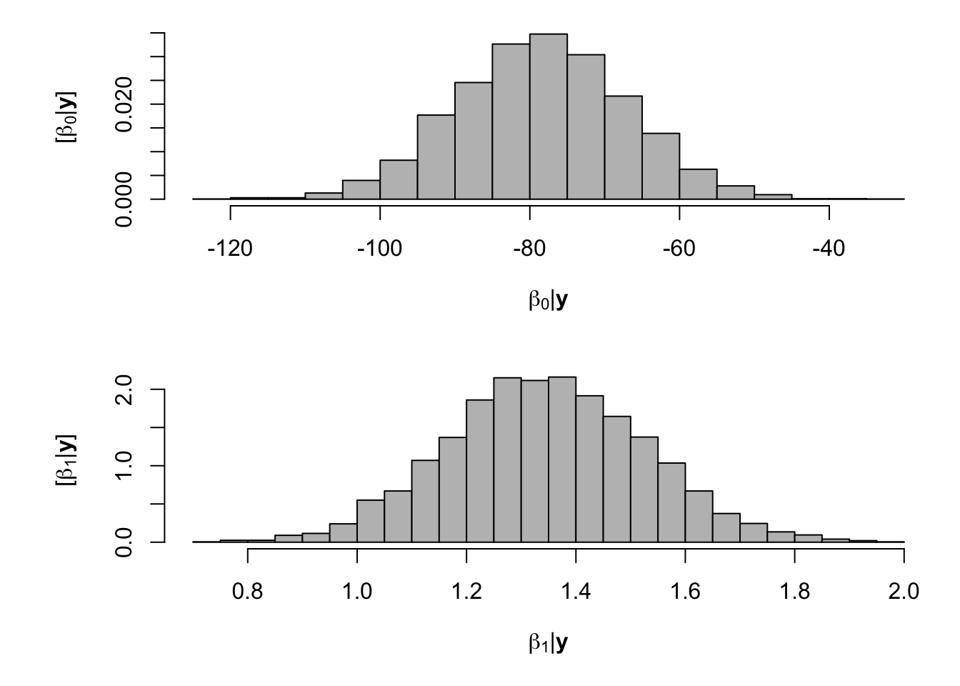
What value of Ndfa is needed to achieve a neutral N balance?
hist(-samples$beta.save[1,-c(1:1000)]/samples$beta.save[2,-c(1:1000)],xlab=expression(theta*"|"*bold(y)),ylab=expression("["*theta*"|"*bold(y)*"]"),freq=FALSE,col="grey",main="",breaks=30)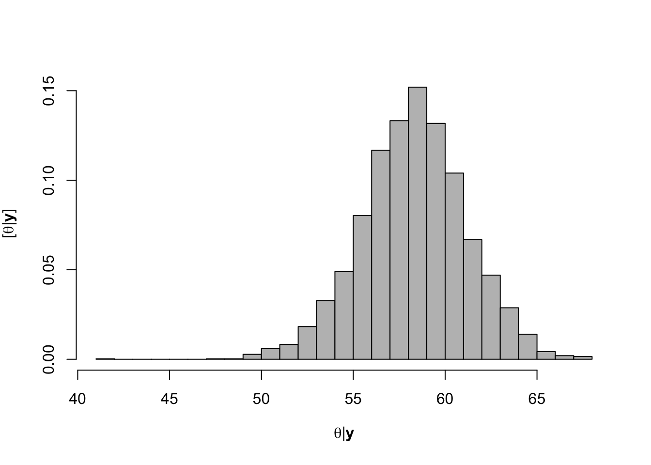
## [1] 58.25093# 95% credible intervals for theta quantile(-samples$beta.save[1,]/samples$beta.save[2,],prob=c(0.025,0.975))## 2.5% 97.5% ## 52.66723 63.72911- Visual representation of posterior distribuiton of theta \(\theta\)
# Plot data and theta
plot(df.fp$Ndfa,df.fp$PartNbalance,
 xlab="Ndfa (%)",ylab="Partial N balance (kg/ha)",
 xlim=c(0,110),ylim=c(-100,200),main="Field pea")
abline(a=0,b=0,col="gold",lwd=3)
abline(v=58.3,lwd=3,lty=2,col="green")
abline(v=52.7,lwd=1,lty=2,col="green")
abline(v=63.7,lwd=1,lty=2,col="green")
rug(-samples$beta.save[1,]/samples$beta.save[2,],col=gray(0.5,0.03))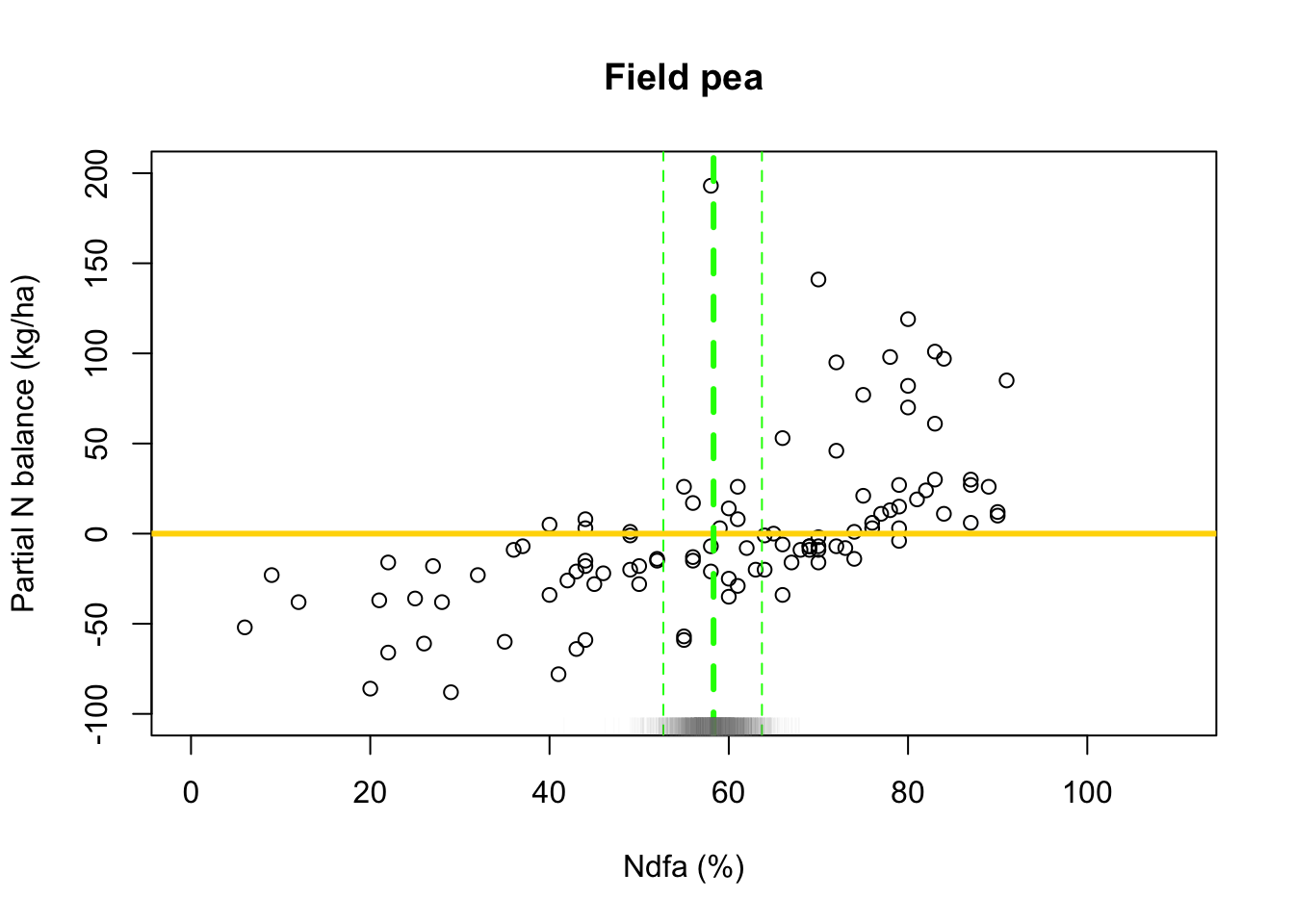
1.9 Low information content data
What value of Ndfa is needed to achieve a neutral N balance?
df.wl <- df.all[which(df.all$Scenario=="Scenario B"),]
plot(df.wl$Ndfa,df.wl$PartNbalance,
 xlab="Ndfa (%)",ylab="Partial N balance (kg/ha)",
 xlim=c(0,110),ylim=c(-100,200),main="White lupin")
abline(a=0,b=0,col="gold",lwd=3)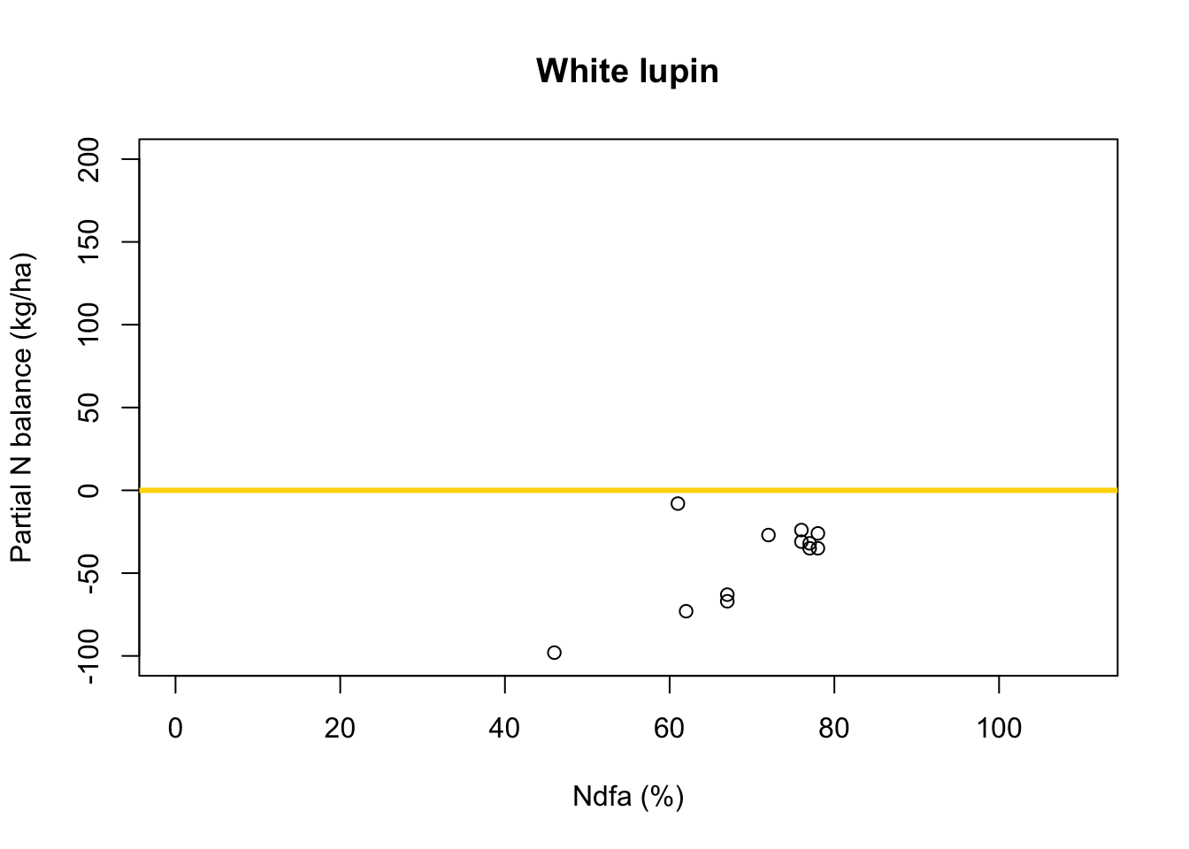
Using least squares
- What value of Ndfa is needed to achieve a neutral N balance?
beta0.hat <- as.numeric(coef(m1)[1])
beta1.hat <- as.numeric(coef(m1)[2])
theta.hat <- -beta0.hat/beta1.hat
theta.hat
## [1] 93.09456- Visual representation of \(\theta\)
# Plot data, line of best fit and theta
plot(df.wl$Ndfa,df.wl$PartNbalance,
 xlab="Ndfa (%)",ylab="Partial N balance (kg/ha)",
 xlim=c(0,110),ylim=c(-100,200),main="White lupin")
abline(a=0,b=0,col="gold",lwd=3)
abline(m1,col="red",lwd=3)
abline(v=93.1,lwd=3,lty=2,col="green")
Using likelihood-based inference
- Fit linear model to data using using maximum likelihood estimation
library(nlme) # Fit simple linear regression model using maximum likelihood estimation m2 <- gls(PartNbalance ~ Ndfa,data=df.wl,method="ML")- What value of Ndfa is needed to achieve a neutral N balance?
# Use maximum likelihood estimate (MLE) to obtain estimate of theta
beta0.hat <- as.numeric(coef(m2)[1])
beta1.hat <- as.numeric(coef(m2)[2])
theta.hat <- -beta0.hat/beta1.hat
theta.hat
## [1] 93.09456# Use delta method to obtain approximate approximate standard errors and # then construct Wald-type confidence intervals library(msm) theta.se <- deltamethod(~-x1/x2, mean=coef(m2), cov=vcov(m2)) theta.ci <- c(theta.hat-1.96*theta.se,theta.hat+1.96*theta.se) theta.ci## [1] 76.91135 109.27778- Visual representation of \(\theta\)
# Plot data, line of best fit and theta
plot(df.wl$Ndfa,df.wl$PartNbalance,
 xlab="Ndfa (%)",ylab="Partial N balance (kg/ha)",
 xlim=c(0,110),ylim=c(-100,200),main="White lupin")
abline(a=0,b=0,col="gold",lwd=3)
abline(m1,col="red",lwd=3)
abline(v=93.1,lwd=3,lty=2,col="green")
abline(v=76.9,lwd=1,lty=2,col="green")
abline(v=109.2,lwd=1,lty=2,col="green")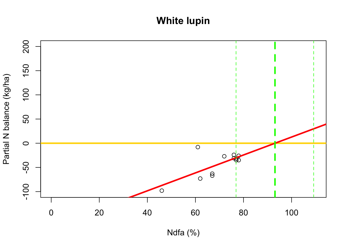
Using Bayesian linear regression
- Assume that \(y_i=\beta_{0}+\beta_{1}x_{i}+\varepsilon_i\) with \(\varepsilon_i\sim \text{N}(0,\sigma^2)\), \(\beta_{0}\sim \text{N}(0,10^6)\) and \(\beta_{1}\sim \text{N}(2.5,0.1)\)
- Model fitting
samples <- norm.reg.mcmc(y = df.wl$PartNbalance,X = model.matrix(~ Ndfa,data=df.wl),
                      beta.mn = c(0,2.5),beta.var=c(10^6,0.1),
                      s2.mn = 10, s2.sd = 10^6,
                      n.mcmc = 5000)

burn.in <- 1000
# Look a histograms of posterior distributions
par(mfrow=c(2,1),mar=c(5,6,1,1))
hist(samples$beta.save[1,-c(1:1000)],xlab=expression(beta[0]*"|"*bold(y)),ylab=expression("["*beta[0]*"|"*bold(y)*"]"),freq=FALSE,col="grey",main="",breaks=30)
hist(samples$beta.save[2,-c(1:1000)],xlab=expression(beta[1]*"|"*bold(y)),ylab=expression("["*beta[1]*"|"*bold(y)*"]"),freq=FALSE,col="grey",main="",breaks=30)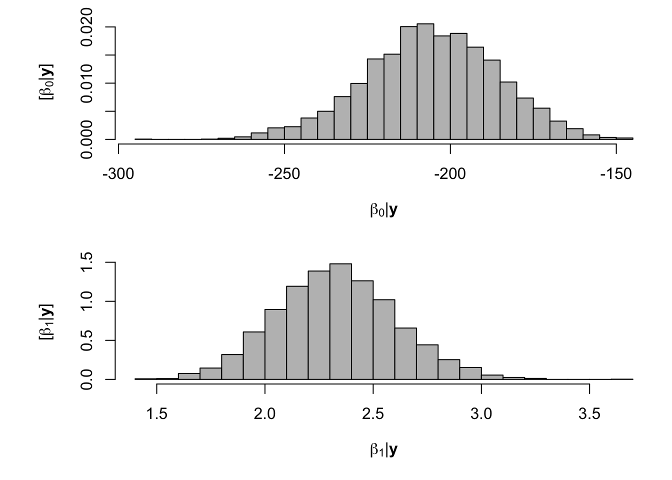
- What value of Ndfa is needed to achieve a neutral N balance?
hist(-samples$beta.save[1,-c(1:1000)]/samples$beta.save[2,-c(1:1000)],xlab=expression(theta*"|"*bold(y)),ylab=expression("["*theta*"|"*bold(y)*"]"),freq=FALSE,col="grey",main="",breaks=30)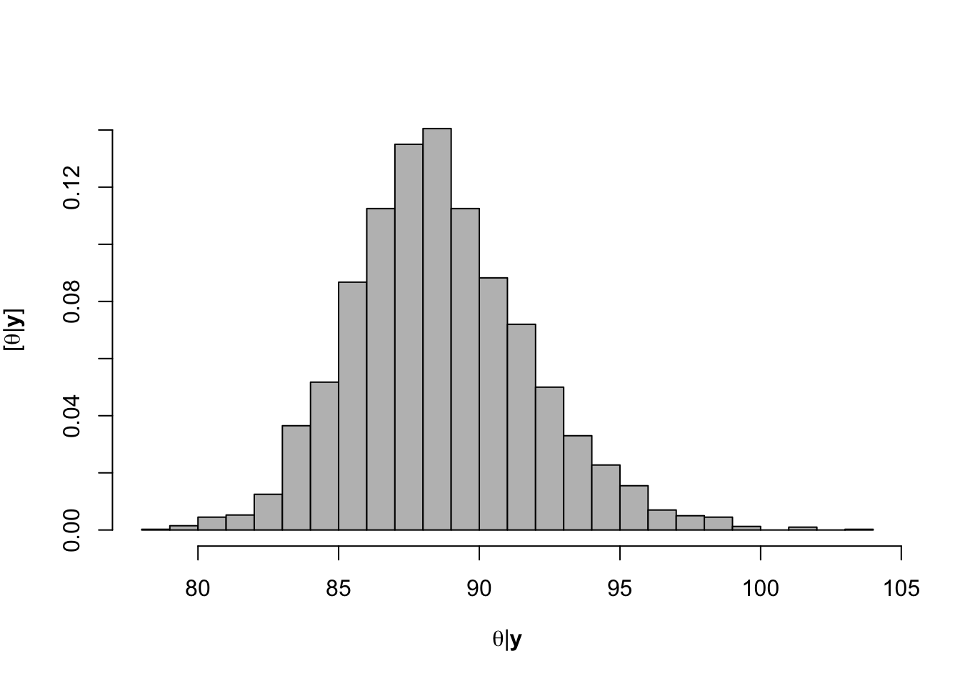
## [1] 88.55595# 95% credible intervals for theta quantile(-samples$beta.save[1,]/samples$beta.save[2,],prob=c(0.025,0.975))## 2.5% 97.5% ## 82.59249 95.51476# Plot data and theta plot(df.wl$Ndfa,df.wl$PartNbalance, xlab="Ndfa (%)",ylab="Partial N balance (kg/ha)", xlim=c(0,110),ylim=c(-100,200),main="Field pea") abline(a=0,b=0,col="gold",lwd=3) abline(v=88.6,lwd=3,lty=2,col="green") abline(v=82.7,lwd=1,lty=2,col="green") abline(v=95.7,lwd=1,lty=2,col="green") rug(-samples$beta.save[1,]/samples$beta.save[2,],col=gray(0.5,0.03))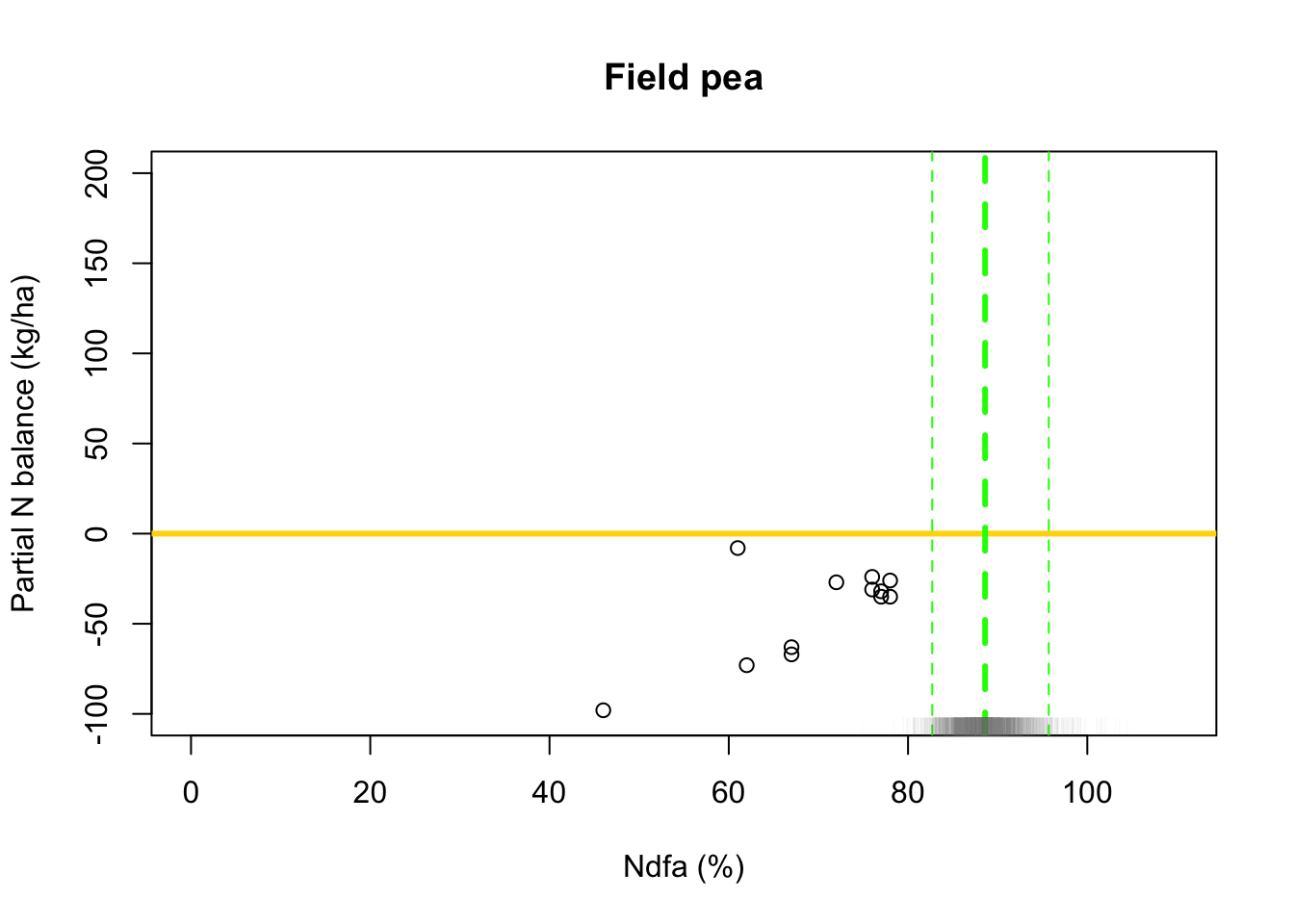
1.10 Summary
- Bayesian models for data analysis are not new
- Bayesian models are very flexible
- Once a Bayesian model is specified (developed) estimation and inference is automatic
- Bayesian model require more assumptions that likelihood-only based models
- Nearly all Bayesian model are fit to data using sampling-based algorithms that are capable of taking random samples from the posterior distribution