3 Day 3 (March 5)
3.1 Review and extension
- “Yesterdays posterior becomes tomorrows prior”
- Back to the coin/phone flip example…
- Download R script here
3.2 Adaptive design
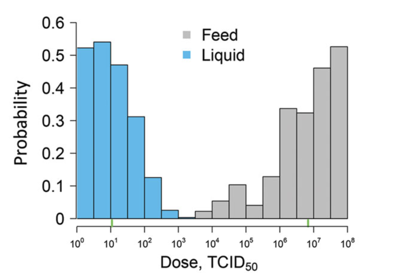
A story and a study (link)

Design elements
- Needed to estimate median infectious dose (ID50) of African Swine Fever Virus with as much precision as possible (i.e., we want to most efficient design)
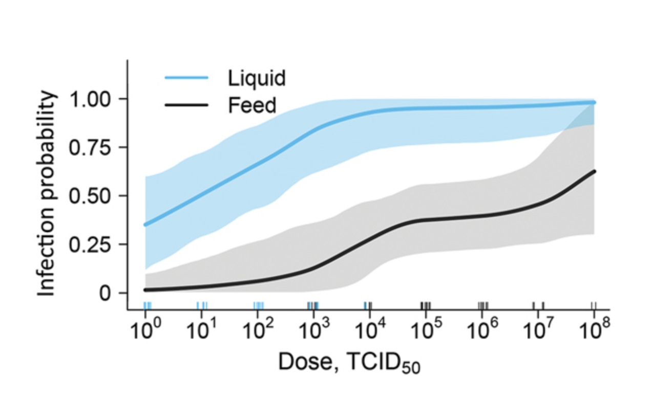
- Mild interest in the dose-response curve
- Big data (n=84 binary responses)!
- Experiment can be conducted simultaneously in two rooms with 7 pigs in each room (i.e., seven opportunities to reassess the design)
- Three different types of tests for ASFV with some giving false negatives
- In addition to dose, two additional “treatments” were if the virus was in the feed or the water of the animal.
- No great guess of what doses should be tried (e.g., something between \(10^0\) and \(10^8\) TCID).
Initial questions I had?
- How do I design an experiment when I don’t know enough about the system to be able to figure out what treatments/dose should be applied.
The model building process (prior to data collection)
- Continual Reassessment Method: A Practical Design for Phase 1 Clinical Trials in Cancer (O’Quigley et al. 1990)
- Occupancy models from ecology but applied to disease data (Davenport et al. 2018)
- Minimal assumptions behind the dose-response using an embed machine learning approach (shape constrained splines; Shaby and Fink 2012)
Required results
- Posterior distributions of the 50% infectious dose
- Posterior distributions of the 50% infectious dose
Bonus Bayesian model results
- Dose response curves
- Multiple exposure link
- False negative rate for the three different ASFV tests which led to new work

- Dose response curves
3.3 Modeling body weight
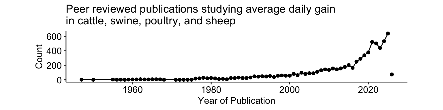
A day in the life of an animal scientist
- In production/industry, the average daily gain is a major response of interest.
- Average daily gain is associated to efficiency and productivity.
- Experiments often compare ADG.
3.3.1 Applied example – Weight of hens
- The common notion in poultry science is that hens show a slight drop in body weight when they are going through puberty (lay their first egg).
- Data below come from 10 hens with weight measured 2 times a week.
Questions:
- Can we test the common belief that hens show a slight drop in body weight? (i.e., ADG < 0)
- Can we estimate the moment they laid their first egg by looking at body weight data?
This is how the data look like:
df <- read.csv("https://raw.githubusercontent.com/jlacasa/miscellaneous/refs/heads/main/data/hens.csv")
head(df)
## hen age bw
## 1 1 143 2004.141
## 2 1 146 2067.207
## 3 1 150 2162.490
## 4 1 153 2280.510
## 5 1 157 2402.646
## 6 1 160 2411.095# compute the ADG
df <- df |>
mutate(bw = bw/1000) |>
group_by(hen) |>
mutate(adg = (bw - lag(bw)) / (age - lag(age)) ) |>
ungroup()
# see how we start losing power by dropping a datapoint
head(df)## # A tibble: 6 × 4
## hen age bw adg
## <int> <int> <dbl> <dbl>
## 1 1 143 2.00 NA
## 2 1 146 2.07 0.0210
## 3 1 150 2.16 0.0238
## 4 1 153 2.28 0.0393
## 5 1 157 2.40 0.0305
## 6 1 160 2.41 0.00282The figures below show the two possible responses: raw data, or the average daily gain.
Statistical modeling
Considering everything we know about animal science and previous approaches to this problem, there are three candidate models to analyze these data.
Model 1:
\[ADG_{ij} \sim N(\mu_{ij}, \sigma^2), \\ \mu_{ij} = \beta_{0} + b_i + T_j,\] where \(\beta_{0}\) is the intercept, \(b_i\) is the effect of the \(i\)th hen, and \(T_j\) is the effect of the \(j\)th time. Note that, in this model, time is considered a categorical factor.
Model 2: \[ADG_{ij} \sim N(\mu_{ij}, \sigma^2), \\ \mu_{ij} = \beta_{0} + b_i + f(t_{ij}),\] where \(\beta_{0}\) is the intercept, \(b_i\) is the effect of the \(i\)th hen, and \(f(t_{ij})\) is a smooth function of time. Note that, in this model, time is considered a continuous factor.
Model 3: \[BW_{ij} \sim N(\mu_{ij}, \sigma^2), \\ \mu_{ij} = \beta_{0} +b_i + f(t_{ij}),\] where \(\beta_{0}\) is the intercept, \(b_i\) is the effect of the \(i\)th hen, and \(f(t_{ij})\) is a smooth function of time. Note that, in this model, time is considered a continuous factor.
Note that in Model 2 and Model 3, the “smooth function of time” can be modeled using B-splines. B-splines are piecewise polynomial functions that can be generally expressed as
\[f(t) = \sum_{l=1}^k B_l^m(t) \beta_l,\] where \(B_l^m(t)\) is a known basis function of order \(m\) that acts locally and \(\beta_l\) is the basis coefficient parameter.
Below is R code to fit those models. We can fit these models using classical statistics:
m1 <- lm(adg ~ factor(hen) + factor(age), data = df)
m2 <- lm(adg ~ factor(hen) + splines::bs(age, df = 14, degree = 3), data = df)
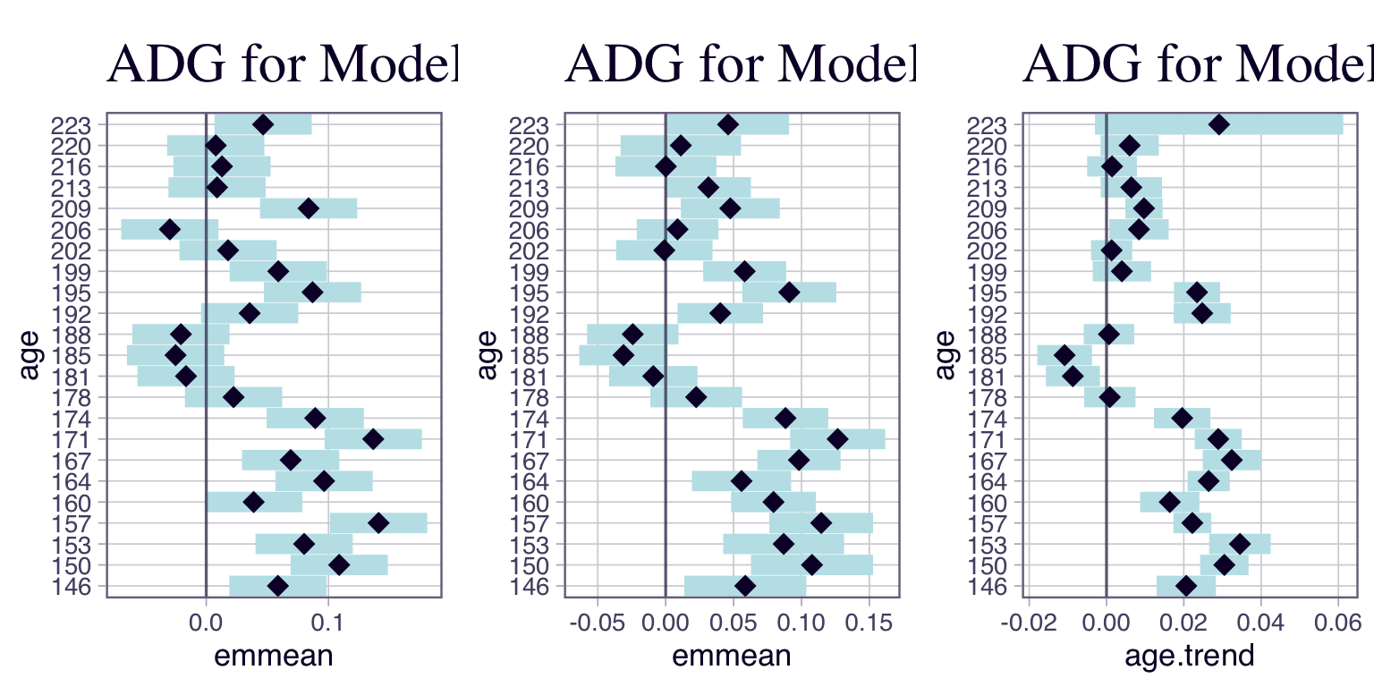
m3 <- lm(bw ~ factor(hen) + splines::bs(age, df = 14, degree = 3), data = df)We can also get the estimated average daily gain. For Model 1 and Model 2, that is just the response. For Model 3, that models body weight, the average daily gain is the slope, \(y = \beta_{0} + f(t) \frac{d y}{d t}\). Note that \(f(t)\) changes depending on \(t\).
Remember that we are looking for \(ADG < 0\). Now, although some point estimates (i.e., at times 181, 185, 188) fulfill this criterion, note that the confidence intervals are telling a more complete story.
Questions:
Can we test the common belief that hens show a slight drop in body weight? (i.e., ADG < 0)
Can we estimate the moment they laid their first egg by looking at body weight data?
What can we conclude about the ADG under the different models (different assumptions)?
3.3.2 Can we estimate the moment they laid their first egg by looking at body weight data AND get uncertainty estimates?
We can fit Model 3, using a few extra assumptions (priors) in a Bayesian framework. You can see the priors in the Stan model below:
\[\beta_0 \sim N(1, 10), \\ b_i \sim N(0, 1), \\ \beta_s \sim N(0,5), \\ \sigma^2 \sim Gamma(10, 0.2).\]
# create spline basis matrix
B <- bs(df$age, df = 14, degree = 3)

# create indicator variables for hen + drop the first level
X_hen <- model.matrix(~ factor(hen), data = df)[, -1]

stan_data <- list(
  N = nrow(df),
  K_hen = ncol(X_hen),
  K_spline = ncol(B),
  bw = df$bw,
  X_hen = X_hen,
  X_spline = B
)

mod <- cmdstan_model("Bsplines.stan")
## [1] "data {"
## [2] " int<lower=0> N; // number of observations"
## [3] " int<lower=1> K_hen; // number of hens (minus 1 for reference)"
## [4] " int<lower=1> K_spline; // number of spline basis functions (df=14)"
## [5] " "
## [6] " vector[N] bw; // response variable"
## [7] " matrix[N, K_hen] X_hen; // indicator variables for hen factor"
## [8] " matrix[N, K_spline] X_spline; // B-spline basis matrix"
## [9] "}"
## [10] ""
## [11] "parameters {"
## [12] " real beta0; // intercept"
## [13] " vector[K_hen] beta_hen; // hen effects "
## [14] " vector[K_spline] beta_spline; // splines coeffs"
## [15] " real<lower=0> sigma; // sigma"
## [16] "}"
## [17] ""
## [18] "model {"
## [19] " "
## [20] " // priors"
## [21] " beta0 ~ normal(1, 10); // intercept (beta_0)"
## [22] " beta_hen ~ normal(0, 1); // priors for hen effects (b_i in model 3) "
## [23] " beta_spline ~ normal(0, 5); // priors for spline coefficients (b_l, a part of f(.) in model 3)"
## [24] " sigma ~ gamma(10, .2); // prior for sigma"
## [25] " "
## [26] " // model"
## [27] " bw ~ normal(beta0 + X_hen * beta_hen + X_spline * beta_spline, sigma);"
## [28] "}"
## [29] ""
## [30] ""fit <- mod$sample(
data = stan_data,
seed = 42,
chains = 3,
parallel_chains = 3,
iter_warmup = 3000,
iter_sampling = 1000,
refresh = 0 # hides sampling progress message
)## Running MCMC with 3 parallel chains...## Chain 1 finished in 0.4 seconds.
## Chain 2 finished in 0.4 seconds.
## Chain 3 finished in 0.4 seconds.
##
## All 3 chains finished successfully.
## Mean chain execution time: 0.4 seconds.
## Total execution time: 0.5 seconds.## # A tibble: 19 × 10
## variable mean median sd mad q5 q95 rhat ess_bulk
## <chr> <dbl> <dbl> <dbl> <dbl> <dbl> <dbl> <dbl> <dbl>
## 1 lp__ 1.89e+2 1.90e+2 3.51 3.55 183. 1.94e+2 1.00 1056.
## 2 beta0 2.01e+0 2.01e+0 0.0173 0.0175 1.98 2.04e+0 1.00 1083.
## 3 beta_hen[1] 1.40e-1 1.40e-1 0.00840 0.00825 0.126 1.53e-1 1.00 2887.
## 4 beta_hen[2] 1.60e-1 1.60e-1 0.00834 0.00813 0.146 1.73e-1 1.000 2882.
## 5 beta_spline[… 4.83e-2 4.89e-2 0.0409 0.0401 -0.0192 1.14e-1 1.00 1783.
## 6 beta_spline[… 1.20e-1 1.20e-1 0.0380 0.0380 0.0577 1.83e-1 1.00 1900.
## 7 beta_spline[… 4.00e-1 4.01e-1 0.0355 0.0341 0.341 4.58e-1 1.00 1596.
## 8 beta_spline[… 4.59e-1 4.59e-1 0.0339 0.0337 0.403 5.14e-1 1.00 1900.
## 9 beta_spline[… 7.02e-1 7.02e-1 0.0338 0.0341 0.646 7.58e-1 1.00 1757.
## 10 beta_spline[… 8.80e-1 8.80e-1 0.0339 0.0334 0.823 9.35e-1 1.00 1695.
## 11 beta_spline[… 8.20e-1 8.20e-1 0.0341 0.0323 0.763 8.76e-1 1.00 1638.
## 12 beta_spline[… 7.22e-1 7.22e-1 0.0336 0.0336 0.667 7.77e-1 1.00 1576.
## 13 beta_spline[… 9.79e-1 9.79e-1 0.0342 0.0338 0.923 1.04e+0 1.00 1794.
## 14 beta_spline[… 9.45e-1 9.45e-1 0.0331 0.0332 0.890 1.00e+0 1.00 1642.
## 15 beta_spline[… 1.02e+0 1.02e+0 0.0339 0.0338 0.964 1.07e+0 1.00 1944.
## 16 beta_spline[… 1.07e+0 1.07e+0 0.0373 0.0373 1.01 1.13e+0 1.00 1710.
## 17 beta_spline[… 1.04e+0 1.04e+0 0.0382 0.0380 0.983 1.11e+0 1.00 2183.
## 18 beta_spline[… 1.11e+0 1.11e+0 0.0233 0.0241 1.07 1.15e+0 1.00 1399.
## 19 sigma 2.87e-2 2.85e-2 0.00312 0.00302 0.0241 3.44e-2 1.00 1995.
## # ℹ 1 more variable: ess_tail <dbl>## Checking sampler transitions treedepth.
## Treedepth satisfactory for all transitions.
##
## Checking sampler transitions for divergences.
## No divergent transitions found.
##
## Checking E-BFMI - sampler transitions HMC potential energy.
## E-BFMI satisfactory.
##
## Rank-normalized split effective sample size satisfactory for all parameters.
##
## Rank-normalized split R-hat values satisfactory for all parameters.
##
## Processing complete, no problems detected.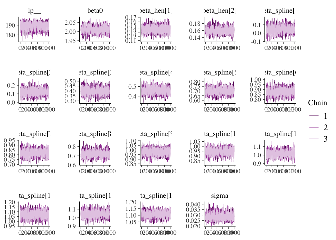
Beyond those estimates, we can also estimate the moment when the slope was negative for the first time.
Note:
- We are quantifying the uncertainty of \(x_{neg}\).
- The shape of the posterior.
- What shape are often assumed in other approximations?
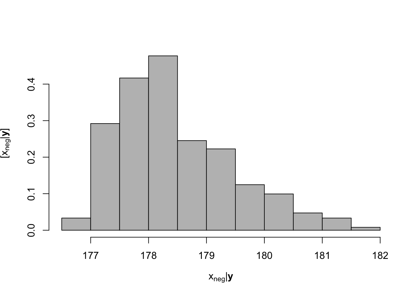
## [1] 178.4745## 2.5% 97.5%
## 177.0741 180.86173.4 Wrap-up
- Questions?
- Further reading
- Ask us because what we recommend will depend on your discipline of study and background in probability theory.
- Further training
- Leave your feedback! Use the QR code below, or this link.

Figure 3.1: QR to access the survey