2 Day 2 (March 4)
2.1 Welcome
- Bonus points for the people who did their homework:
- Think of the assumptions behind ANOVA
- Think about 2 aspects of ANOVA that are positive/useful in your research
- Think about 2 aspects of ANOVA that have challenged you in your research
2.2 What will we learn today?
- Review of classical ANOVA
- An introduction to a multilevel approach to ANOVA
- Applied example and fun facts about bacteria and biofilms
2.3 Why do we need designed experiments?
- Golden rules: replication, randomization, local control
](figures/fishers_diagram.jpg)
Figure 2.1: Fisher’s diagram ‘The Principles of Field Experimentation’. Figure 1 in Preece (1990)
- And why do we need statistics to analyze our experiment results?
- History of designed experiments [link]
Discuss:
- The need for controlled conditions in designed experiments.
- The need to clearly define our research questions.
- Treatment structure, design structure.
2.3.1 On the importance of prior knowledge and of expert “nonstatistical” knowledge
Classical textbooks in designed experiments highlight the importance of prior knowledge and of expert “nonstatistical” knowledge. Use it!
How to use statistical techniques
- Find out as much as you can about the problem
- Don’t forget nonstatistical knowledge
- When you are doing “statistics” do not neglect what you and your colleagues know about the subject matter field. Statistical techniques are useless unless combined with appropriate subject matter knowledge and experience. They are an adjunct to, not a replacement for, subject matter expertise.
- Define objectives.
Chapter 2 in Box, Hunter and Hunter.
“[E]xperimental design and data analysis are different ends of the same process. (…) experiments are designed in a certain way so that useful analyses can be made of the data that will emerge. To discuss one without the other is to play Hamlet without the Prince of Denmark. Before designing an experiment on substances a, b, c and d, some explanation is needed of the supposed relationship between them.”
2.4 Review of classical ANOVA
- The analysis of variance (ANOVA) is one of the most widespread statistical techniques used to analyzed data generated by designed experiments.
- Major advantages:
- Exploratory data analysis
- Answers the question “is this batch of coefficients significant (with \(\alpha =\) some number) or not?”
2.4.1 ANOVA is a special case of the general linear model
ANOVA is a special case of the general linear model, where the predictors are categorical variables. Let’s consider the following scenario:
A group of scientists wants to study the effects of 2 treatment factors, \(A\) and \(C\), on their response. They run an experiment where all experimental units are independent (aka completely randomized design). A good model to represent the data generating process can be
\[y_{ijk} = \mu_0 + A_i + C_j +AC_{ij} + \varepsilon_{ijk}, \\ \varepsilon_{ijk} \sim N(0,\sigma^2),\]
or
\[y_{ijk} \sim N(\mu_{ijk},\sigma^2), \\ \mu_{ijk} = \mu_0 + A_i + C_j +AC_{ij},\]
where \(y_{ijk}\) is the observation of the \(i\)th A treatment, \(j\)th C treatment, and \(k\)th repetition, \(\mu_{ijk}\) is the mean for that observation and is the sum of the overall mean \(\mu_0\), the effect of the \(i\)th level of \(A\), the effect of the \(j\)th level of \(C\), the effect of the \(i\)th level of \(A\) and the \(j\)th level of \(C\).
- Note that the effects in the model above are all the \(A_i\)s, all the \(C_j\)s, and all the \(AC_{ij}\)s.
- The ANOVA equivalent to the model above more explicitly divides these coefficients in batches, called “Sources of variability”.
Table 1. Classical analysis of variance table for a two-way treatment structure in a completely randomized design. Source = source of variation; df = degrees of freedom; EMS = expected mean squares; SS = sums of squares; F = F statistic; p-value = P(F statistic > critical F under \(H_0\) ).
| Source | df | EMS | SS | F | p-value |
|---|---|---|---|---|---|
| A | \(a - 1\) | \(\sigma^2_\varepsilon + \phi^2(\alpha)\) | \(SS_A = \sum_{i=1}^a n_i(\hat{y}_{i\cdot} - \hat{y}_{\cdot\cdot})^2\) | \(F_A^{\star} = \frac{MS_{A}}{MSE}\) | \(P(F^{\star}_A >F)\) |
| C | \(c - 1\) | \(\sigma^2_\varepsilon + \phi^2(\gamma)\) | \(SS_C = \sum_{j=1}^c n_j(\hat{y}_{\cdot j} - \hat{y}_{\cdot\cdot})^2\) | \(F_C^{\star} = \frac{MS_{C}}{MSE}\) | \(P(F^{\star}_C >F)\) |
| A \(\times\) C | \((a-1)(c-1)\) | \(\sigma^2_\varepsilon + \phi^2(\alpha \gamma)\) | \(SS_{A \times C} = \sum_{i=1}^a \sum_{j=1}^c n_i n_j(\hat{y}_{i j} - \hat{y}_{\cdot\cdot})^2\) | \(F_{A \times C}^{\star} = \frac{MS_{A\times C}}{MSE}\) | \(P(F^{\star}_{A \times C} >F)\) |
| Error | \(N-ac\) | \(\sigma^2_\varepsilon\) | \(SSE = \sum_{i=1}^{n}(y_i-\hat{y_i})^2\) |
What are the different columns doing?
- Source of variability: This column is equivalent to the components in the linear predictor of our general linear model.
- Expected mean squares (EMS) consist of the sum of:
- The residual variance, \(\sigma^2_\varepsilon\),
- \(\phi^2(\alpha)\), \(\phi^2(\gamma)\) and \(\phi^2(\alpha \gamma)\): Quadratic functions of the main effect means. Note that \(\phi^2(\cdot) = 0\) when effects don’t exist (zero effects).
- There’s an EMS for each source of variability.
- Sums of squares (SS) represent the decomposition of the total sums of squares, divided into what corresponds to each batch.
- Mean square is the SS divided by degrees of freedom for that source. \(MSE\) is the mean squared error, \(MSE = \frac{SSE}{df_e}\) and is also equivalent to \(\hat{\sigma}^2\).
- The F test statistic \(F^\star_m\) is the ratio \(MS_m / MSE\).
- The p-value corresponds to the hypothesis test testing whether \(F^\star_m>F_{m}\). In this context, \(F_{crit}\) is a value corresponding to the distribution \(F_{df_{numerator}, df_{denominator}}\) with noncentrality parameter 0. The noncentrality parameter is 0 because our \(H_0\) in this case is \(\phi^2(\alpha) = 0\) and thus, for example, \(MS_A = \sigma^2_\varepsilon + \phi^2(\alpha) = \sigma^2_\varepsilon + 0\). This means that under \(H_0\), \(MS_A =MSE\).
2.4.2 Interpreting classical ANOVA
- Testing row by row whether the effects \(A\), \(C\), and/or \(A \times C\) are “statistically significant”.
- Two possible outcomes: We reject \(H_0\), or we don’t reject \(H_0\). WE DON’T CONFIRM \(H_0\).
- We select a significant \(\alpha\) type I error we feel comfortable with.
- In this context, the opposite to some effect being “statistically significant” (\(p<\alpha\)) means that there is not enough evidence to say that there is an effect!
ANOVA is a simultaneous test on several linear combinations:
We use several \(\mathbf{K}\) matrices that, if \(\mathbf{K}'\boldsymbol{\beta}=0\), \(A_1 =A_2 = \dots = A_a\). Assume \(a=4\), a possible \(\mathbf{K}\) matrices is
\[\mathbf{K}' = \begin{bmatrix} 0 & 1 & 0 & 0 & -1 & 0 & \dots & 0 \\ 0 & 0 & 1 & 0 & -1 & 0 & \dots & 0 \\ 0 & 0 & 0 & 1 & -1 & 0 & \dots & 0 \end{bmatrix}.\]
Now assume \(b=3\), a possible \(\mathbf{K}\) matrices is
\[\mathbf{K}' = \begin{bmatrix} 0 & 0 & 0 & 0 & 0 & 1 & 0 & -1 & 0 & \dots & 0 \\ 0 & 0 & 0 & 0 & 0 & 0 & 1 & -1 & 0 & \dots & 0 \\ 0 & 0 & 0 & 0 & 0 & 0 & 0 & -1 & 0 & \dots & 0 \end{bmatrix}.\]
Note:
- The first column is the overall mean \(\mu_0\).
- Each one of these \(\mathbf{K}\) matrices goes into a single line of the ANOVA.
- The rows must be mutually independent but not necessarily mutually orthogonal.
- This approach is helpful for distributions beyond the Normal.
- Inference is not simultaneous, but line-by-line: each hypothesis test is evaluated independently.
- All we get from ANOVAs are yes-or-no answers about there is enough evidence to say whether whatever factor was important or not.
2.4.3 Changing the structure in the data
The model above,
\[y_{ijk} \sim N(\mu_{ijk},\sigma^2), \\ \mu_{ijk} = \mu_0 + A_i + C_j +AC_{ij},\]
assumes iid (independent and identically distributed) data. This type of assumption is typical of a completely randomized design, where all experimental units are independent. This assumption stops being appropriate once the experiment logistics have some more complexity to them.
2.4.4 A split-plot example
Let’s take the same example we used before:
A group of scientists wants to study the effects of 2 treatment factors, \(A\) and \(C\), on their response.
They run an experiment where all experimental units are independent (aka completely randomized design).
Because of practical restrictions, they run an experiment where experimental units of \(A\) and \(C\) have different dimensions.
This results in a design that looks like
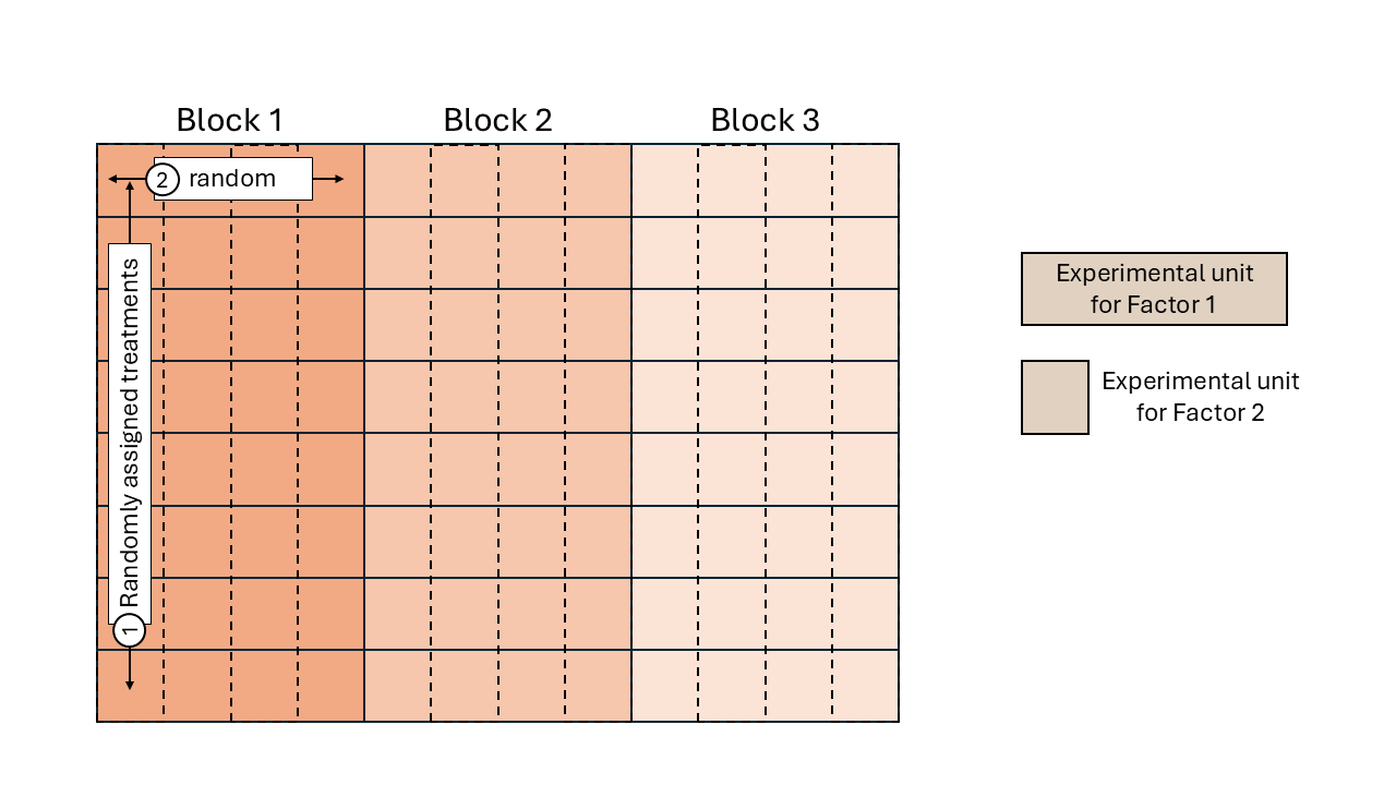
Figure 2.2: Schematic representation of a split-plot design.
A good model to represent the data generating process can be
\[y_{ijk} \vert \boldsymbol{u} \sim N(\mu_{ijk},\sigma^2), \\ \mu_{ijk} = \mu_0 + b_k + A_i + w_{i(k)} + C_j +AC_{ij}, \\ b_k \sim N(0, \sigma^2_b), w_{i(k)} \sim N(0, \sigma^2_w)\]
where \(y_{ijk}\) is the observation of the \(i\)th treatment A, \(j\)th treatment C, and \(k\)th repetition, \(\mu_{ijk}\) is the mean for that observation and is the sum of the overall mean \(\mu_0\), the effect of the \(i\)th level of \(A\), the effect of the \(j\)th level of \(C\), the effect of the \(i\)th level of \(A\) and the \(j\)th level of \(C\).
Table 2. Classical analysis of variance table for a two-way treatment structure for a split-plot in a completely randomized design structure. Source = source of variation; df = degrees of freedom; EMS = expected mean squares; SS = sums of squares; F = F statistic; p-value = P(F statistic > critical F under \(H_0\) ).
| Source | df | EMS | SS | F | p-value |
|---|---|---|---|---|---|
| Block | \(b - 1\) | \(\sigma^2_\varepsilon + c \sigma^2_{wp} + ac \sigma^2_b\) | |||
| A | \(a - 1\) | \(\sigma^2_\varepsilon + c \sigma^2_{wp} + \phi^2(\alpha)\) | \(SS_A = \sum_{i=1}^a n_i(\hat{y}_{i\cdot} - \hat{y}_{\cdot\cdot})^2\) | \(F_A^{\star} = \frac{MS_{A}}{MSE}\) | \(P(F^{\star}_{A} >F)\) |
| Whole plot | \((b-1)(a - 1)\) | \(\sigma^2_\varepsilon + c \sigma^2_{wp}\) | |||
| C | \(c - 1\) | \(\sigma^2_\varepsilon + \phi^2(\gamma)\) | \(SS_C = \sum_{j=1}^c n_j(\hat{y}_{\cdot j} - \hat{y}_{\cdot\cdot})^2\) | \(F_C^{\star} = \frac{MS_{C}}{MSE}\) | \(P(F^{\star}_{C} >F)\) |
| A \(\times\) C | \((a-1)(c-1)\) | \(\sigma^2_\varepsilon + \phi^2(\alpha \gamma)\) | \(SS_{A \times C} = \sum_{i=1}^a \sum_{j=1}^c n_i n_j(\hat{y}_{i j} - \hat{y}_{\cdot\cdot})^2\) | \(F_{A \times C}^{\star} = \frac{MS_{A\times C}}{MSE}\) | \(P(F^{\star}_{A \times C} >F)\) |
| Error | \(a(b-1)(c-1)\) | \(\sigma^2_\varepsilon\) | \(SSE = \sum_{i=1}^{n}(y_i-\hat{y_i})^2\) |
2.4.5 Other structures in the data
- How would you design the ANOVA table for incomplete, unbalanced data?
- How do you determine the degrees of freedom of the different levels?
2.4.6 Criticism to ANOVA
Perhaps best summarized here:
“Econometricians see [ANOVA] as an uninteresting special case of linear regression. Bayesians see [ANOVA] as an inflexible classical method. Theoretical statisticians have supplied many mathematical definitions [see, e.g., Speed (1987)]. Instructors see [ANOVA] as one of the hardest topics in classical statistics to teach, especially in its more elaborate forms such as split-plot analysis.”
In summary:
ANOVA is perhaps one of the most common models used to analyze data generated by designed experiments.
Appealing to scientists because it involves mostly easy computations.
But do easy computations = easy inference?
Assumptions: independence, normality.
ANOVA asks questions that may not be our research question
ANOVA gives answers that may not be our goal
ANOVA relies on assumptions that may not be appropriate for our data generating process
For some structures in the data, it may be hard to write out the ANOVA shell
2.5 A multilevel approach to ANOVA
- Contains the ideas of classical ANOVA that are appealing to scientists:
- Exploratory data analysis
- Detection of “important” factors
- Aim to solve some of the less useful aspects of ANOVA:
- Simultaneous inference (i.e., no longer interpreting row-by-row)
- Inference on the relative importance of factors (SS in classical ANOVA are not interpretable)
- Simultaneous inference (i.e., no longer interpreting row-by-row)
Recall the previous model
\[y_{ijk} = \mu_0 + A_i + C_j +AC_{ij} + \varepsilon_{ijk}, \\ \varepsilon_{ijk} \sim N(0,\sigma^2).\]
- Consider \(A_i, C_j, AC_{ij}\) are batches of coefficients.
- Use the notation \(\mu_{ijk} = \mathbf{X} \boldsymbol{\beta}\).
- Now, let’s assume \(A_i \sim N(0, \sigma^2_{A}), \ C_j \sim N(0, \sigma^2_{C}), AC_{ij} \sim N(0, \sigma^2_{AC})\)
- Using general notation: \[\beta^{(m)}_j\sim N(0, \sigma^2_m).\]
Let’s take 5 to interpret \(\sigma^2_m\)
Our priors on each \(\sigma^2_m\) reflect the level of treatment difference we’d expect to see. A noninformative prior could be \[\sigma^2_m \sim \text{Inv-}\chi^2(\nu_m, \sigma^2_{0m}),\] where \(\nu_m\) is the degrees of freedom corresponding to batch \(m\), and \(\sigma^2_{0m} = 0\).
Note: For values of in which \(J_m\) is large (i.e., rows of the ANOVA table corresponding to many to many linear predictors), \(\sigma_m\) is essentially estimated from data. When \(J_m\) is small, the flat prior distribution implies that is allowed the possibility of taking on large values, which minimizes the amount of shrinkage in the effect estimates.
We further quantify the importance of batch \(m\) using
\[s_m = \sqrt{\frac{1}{df_m} \beta^{(m)T} [I-C^{(m)} (C^{(m)T} C^{(m)})^{-1}C^{(m)T} ] \beta^{(m)} },\] which is equivalent to taking the standard deviation of the different \(\beta_j\)s.
2.5.1 \(\sigma^2_m\) and \(s^2_m\)
In so many words, we get two quantities that describe the effect sizes of the different treatment factors.
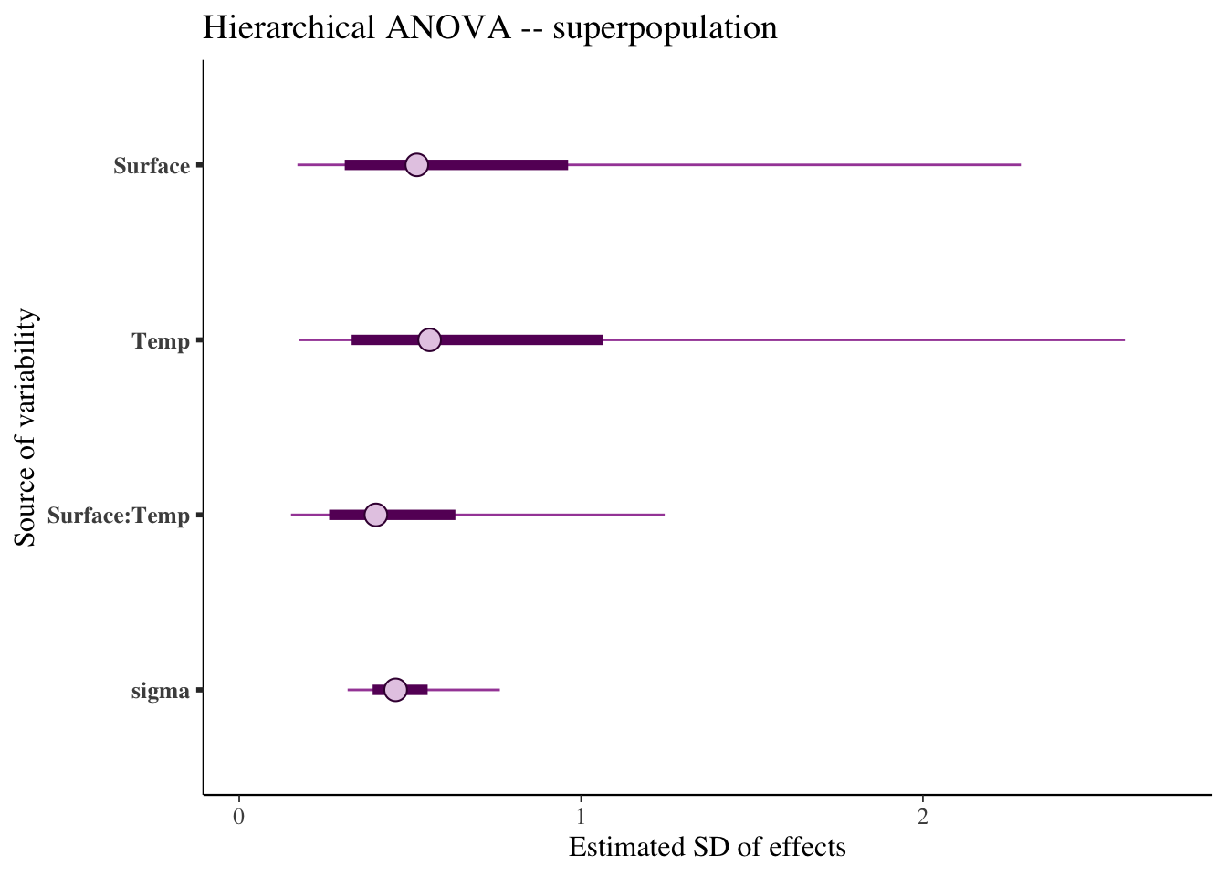
- \(\sigma^2_m\) includes the uncertainty of observing new levels (superpopulation),
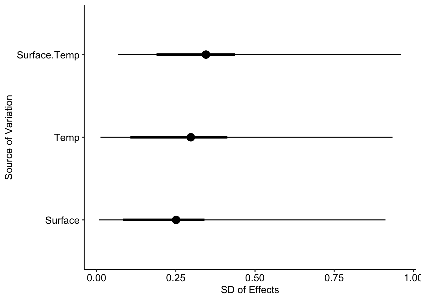
- \(s^2_m\) only includes the differences between the levels present in the data (finite population).
2.6 Review
- Classical ANOVA \(H_0: A_1 = A_2 = \dots = A_a; \ H_a = \text{at least one } A_i \neq A_{i'}\).
- Multi-level ANOVA divides all predictors in batches that are modeled \(\beta^{(m)}_j\sim N(0, \sigma^2_m)\).
- Inference from \(\beta^{(m)}_j\), \(\sigma^2_m\), \(SD(\beta^{(m)}_j)\).
- Determining the structure in the error becomes less critical.
2.7 Applied example
The data below were generated by an experiment in microbiology that aimed to study the growth of Lysteria monocyogenes and Pseudonomas fluorescens in biofilm formation on two different surfaces and under two different temperatures. The experiment was run under a completely randomized design (CRD).
]](figures/Biofilm-Infographic-2048x1229.jpg)
Figure 2.3: Schematic representation of Biofilm formation. [Link to image source]
Experiment main objective
The scientists that ran this experiment are interested in evaluating (i) the differences in biofilm formation between temperatures, and (ii) the differences in biofilm formation across surfaces.
Prior information
- Greater temperatures promote bacteria growth.
- Biofilm formation differs depending on the surface.
dat <- read.csv("https://raw.githubusercontent.com/jlacasa/miscellaneous/refs/heads/main/data/lysteria_growth.csv")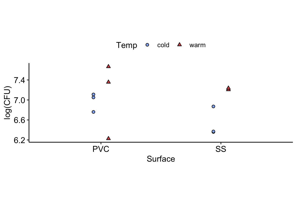
The model corresponding these data is typically
\[y_{ijk} \sim N(\mu_{ijk},\sigma^2), \\ \mu_{ijk} = \mu_0 + A_i + C_j +AC_{ij}.\]
Given our prior information and using the notation \(\mu_{ijk} = \mathbf{X} \boldsymbol{\beta}\), we can say that
\[\beta^{(m)}_j\sim N(0, \sigma^2_m),\] and \[\sigma^2_m \sim \text{Inv-}\chi^2(1, \sigma^2_{0m}).\]
2.7.1 Software implementation
Below is brms code to fit the model described above.
Note that, for now, we are modeling
- \(y \sim N(\mu, \sigma^2_y)\),
- \(\beta_j^{(m)}\sim N(0, \sigma^2_m)\), \(\sigma^2_m \sim \text{Inv- }\chi^2(1)\), and \(\sigma^2_y \sim Gamma(10, 0.5)\).
multilevel_anova <-
brm(
#specify the linear predictor
log_CFU ~ 1 + (1|Surface) + (1|Temp) + (1 | Surface:Temp),
# assign priors to all parameters
prior = c(
# set all sd from an inverse chi sq with their respective DF
# in this case, all treatment factors had the same DF
set_prior("inv_chi_square(1)", class = "sd", group = "Surface", lb=0),
set_prior("inv_chi_square(1)", class = "sd", group = "Temp", lb=0),
set_prior("inv_chi_square(1)", class = "sd", group = "Surface:Temp", lb=0),
# set the prior for the variance
set_prior("gamma(10,0.5)", class = "sd", lb=0)),
# cmstanr is the lightweight version of rstan
backend = "cmdstanr",
# iterations
iter = 6000,
warmup = 5000,
# this depends on your computer
cores = 3,
chains = 3,
# for reproducibility
seed = 42,
# miscellaneous sampler options
control = list(adapt_delta = .9),
# avoid messages of sampling progress
silent = 2,
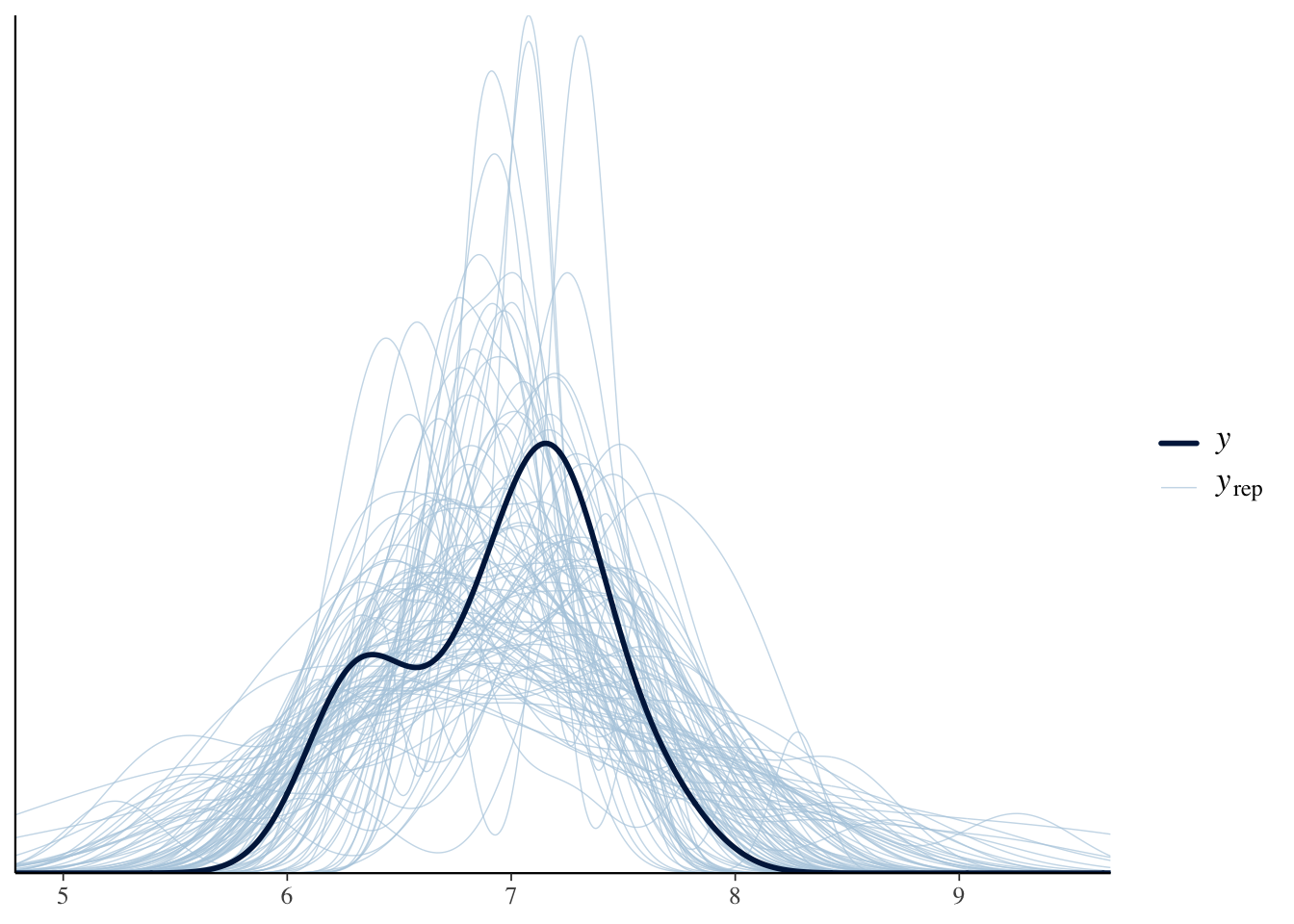
data = dat)After model fitting, we need to make sure that the sampler reached the stationary distribution. Some visual and quantitative model checks:
##  Family: gaussian
##   Links: mu = identity
## Formula: log_CFU ~ 1 + (1 | Surface) + (1 | Temp) + (1 | Surface:Temp)
##    Data: dat (Number of observations: 12)
##   Draws: 3 chains, each with iter = 6000; warmup = 5000; thin = 1;
##          total post-warmup draws = 3000
##
## Multilevel Hyperparameters:
## ~Surface (Number of levels: 2)
##               Estimate Est.Error l-95% CI u-95% CI Rhat Bulk_ESS Tail_ESS
## sd(Intercept)     0.79      0.80     0.14     3.16 1.00     1256      766
##
## ~Surface:Temp (Number of levels: 4)
##               Estimate Est.Error l-95% CI u-95% CI Rhat Bulk_ESS Tail_ESS
## sd(Intercept)     0.52      0.40     0.13     1.61 1.00     1914     1730
##
## ~Temp (Number of levels: 2)
##               Estimate Est.Error l-95% CI u-95% CI Rhat Bulk_ESS Tail_ESS
## sd(Intercept)     0.87      0.89     0.14     3.50 1.00     1687     1349
##
## Regression Coefficients:
##           Estimate Est.Error l-95% CI u-95% CI Rhat Bulk_ESS Tail_ESS
## Intercept     6.96      0.91     4.95     8.80 1.00     1024      804
##
## Further Distributional Parameters:
##       Estimate Est.Error l-95% CI u-95% CI Rhat Bulk_ESS Tail_ESS
## sigma     0.49      0.14     0.30     0.84 1.00     1897     1764
##
## Draws were sampled using sample(hmc). For each parameter, Bulk_ESS
## and Tail_ESS are effective sample size measures, and Rhat is the potential
## scale reduction factor on split chains (at convergence, Rhat = 1).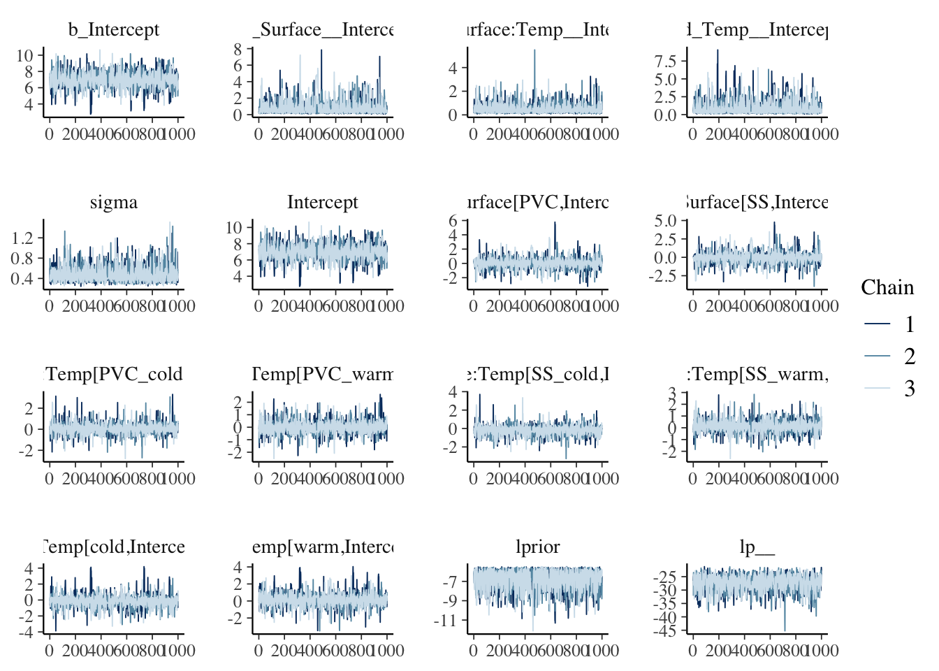
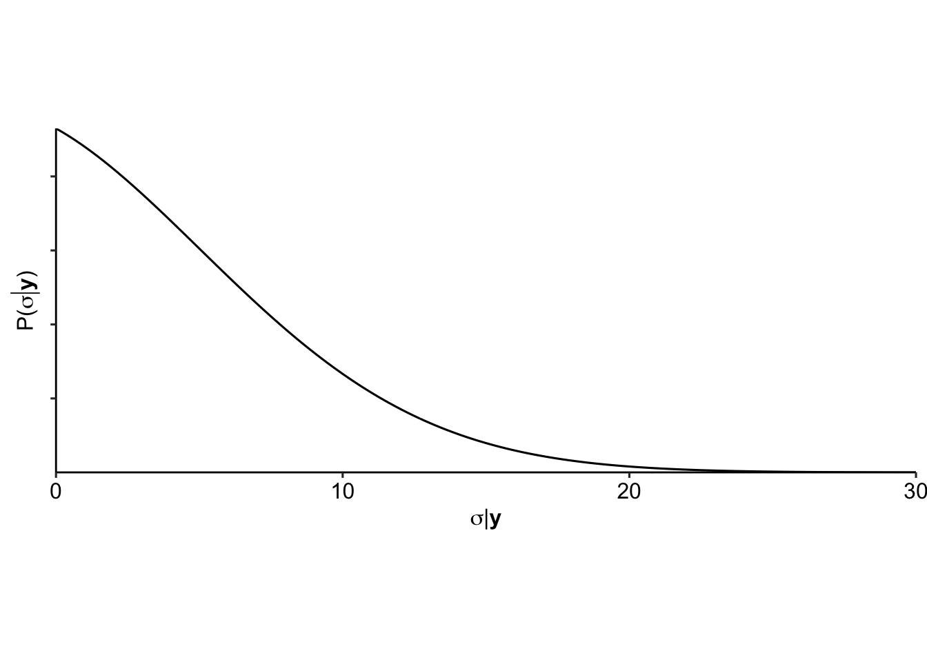
We can now investigate the variances for the superpopulation \(\sigma^2_m\):
And the variances for the finite population \(s^2_m\):
2.7.2 Inference
So far, the inference we can take out of this includes:
- What are the most important treatment factors?
- How important are they?
- What are the estimated means then?
- What is the probability of having 7 logCFU or more?
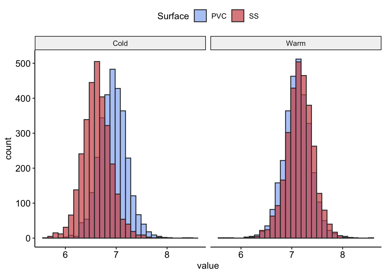
| Surface | Temperature | P(logCFU<7) |
|---|---|---|
| PVC | Cold | 0.60 |
| PVC | Warm | 0.33 |
| SS | Cold | 0.92 |
| SS | Warm | 0.26 |
Let’s compare this with the inference from classical ANOVA
## Anova Table (Type II tests)
##
## Response: log_CFU
##               Sum Sq Df F value Pr(>F)
## Surface      0.07053  1  0.4061 0.5418
## Temp         0.47091  1  2.7111 0.1383
## Surface:Temp 0.24653  1  1.4193 0.2677
## Residuals    1.38960  8
2.8 Wrap-up
- On Monday, we learned how statistical methods with increasing assumptions can give us enhanced inference.
- Today, we learned how those increasing assumptions can give us enhanced inference, even for classical methods like ANOVA.
- Our multilevel ANOVA allows us to make inference at the treatment means level and at the \(s^2_m\) level.